home |
electronics |
toolbox |
science club |
tuxtalk |
photos |
e-cards |
online-shop

kinematic: derivatives and integration in physics
High school physics teaches the kinematic equations as a set of simple formulas:
v = v0 + a0Δt
x = x0 + ½ (v0 + v)Δt = x0 + v0Δt + ½ a0Δt2
v2 = (v0)2 + 2a0Δx
Most school books will show "a" instead of "a0" but the meaning is the same.
Unfortunately it is rarely mentioned that those simplified
formulas are only applicable in special cases. The real formulas are even more simple and easier to remember than
those taught in high school but they require a bit of higher math. You don't need
to be a calculus whiz to get the idea behind the real formulas.
An object sitting at a fixed position has zero velocity. If you move it then it will have a certain velocity
dependent on how fast it moves. In other words the change of position over time is velocity. If you plot
the position x over time then the slope of that position over time curve is the velocity.
x(t) is the equation of the position over time curve. The slope of a curve is mathematically the derivative of the function describing that curve. It is written like this:
        ∂x(t)
v(t) = -------
        ∂t
The short notation is to put a dot on top of x(t) to mean the derivative. I don't have a dot in HTML therefore
I use a dash:
                 ∂x(t)
v(t) =  x'(t) = -------
                 ∂t
This simply a "funny notation" to say: draw the position (x) as a function of time, x(t), and measure the slope. The result is
the velocity as a function of time. In other words change in position is related to velocity.
A change in velocity requires acceleration (or breaking=negative acceleration). Thus the slope of the velocity curve over time is acceleration over time:
                ∂v(t)              ∂2x(t)
a(t) = v'(t) = -------  = x"(t) = --------
                ∂t                 ∂t2
The reverse of a derivative is an integral. In graphical terms that is the area under a curve.
For example a car driving with the constant speed of 2m/s (two meters per second):
v(t) = 2 m/s (blue line in the graph below).
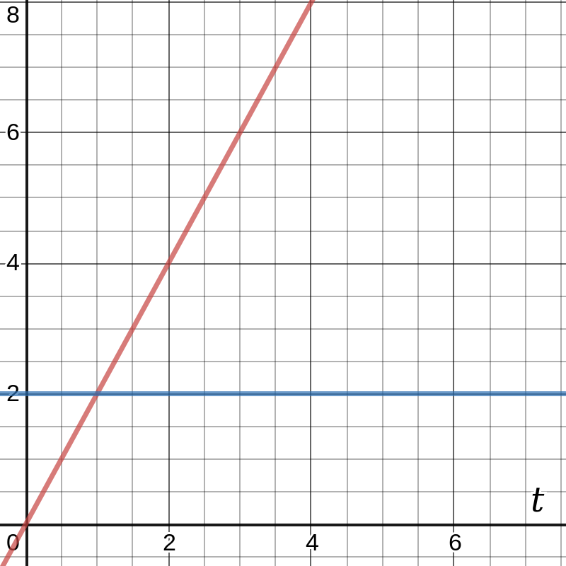
The area under this blue line is a rectangle and it increases as you move to the right of the graph.
This area corresponds to the position of our car. At t=2s the area is 2s*2m/s=4m, at t=3s the area is 2m/s*3s=6m.
x(t) = 2 t
If we draw 2*t into the graph then we get the red line. This is the position of the car over time.
This area under the velocity curve is called in mathematical terms an integral and written as:
x(t) = ∫v(t)∂t
The accumulated area over time under the velocity is the position. This is the reverse of "the change in position is velocity".
Change in velocity was acceleration and the reverse function would be "the area under the acceleration curve is velocity:
v(t) = ∫a(t)∂t
The kinimatic equations as derivatives and integrals
                ∂x(t)
v(t) = x'(t) = -------
                ∂t

                ∂v(t)              ∂2x(t)
a(t) = v'(t) = -------  = x"(t) = --------
                ∂t                 ∂t2

and the reverse functions:

x(t) = ∫v(t)∂t + x0 = ∫∫a(t)∂t2 + x0

v(t) = ∫a(t)∂t + v0
Derivatives and integrals of some basic functions
To use this we have to know how to calculate the derivative or integral of a given function. For
high school level physics you will only need to know the following.
                                           ∂f(t)
function: f(t) = t2 , derivative: f'(t) = -------   = 2 t
                                           ∂t

                                           ∂f(t)
function: f(t) = 2 t, derivative: f'(t) = -------   = 2
                                           ∂t

function: f(t) = constant, derivative: f'(t) = 0
In general the derivative of f(t) = tz is f'(t) = z*tz-1. That is: you put the exponent in front and decrease it by 1.
The integral is the reverse operation of the derivative.
function: f(t) =  t, integral: ∫f(t)∂t = ½ t2

function: f(t) =  constant, integral: ∫f(t)∂t = constant * t
In general the integral of f(t) = tz is ∫f(t) = 1/(z+1) * tz+1. That is: you increase the exponent by one and divide by the value of the new exponent.
The following diagram contains 3 graphs:
f1(t) = 2 (blue line)
f2(t) = 2 t (red line)
f3(t) = t2 (green line)
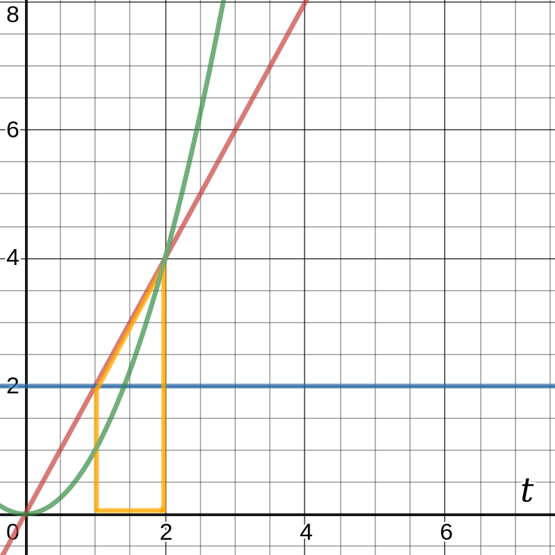
The graphs were chosen such that:
∫f1(t) = f2(t) and ∫f2(t) = f3(t)
The integral of f2(t) is f3(t) but the value of f3 at a given point t is the area
under the line f2(t) starting at t=0. If you want to know the size of the orange area under the red line, from t=1 to t=2 then you have to subtract: f3(2) - f3(1) = 22 - 12 = 3.
The integral of function f2 (∫f2∂t) from t=1 to t=2 is 3.
How to get from our generic kinematic equations to the high school formulas?
The high school formulas mentioned at the top of the page work only under two assumptions:
- acceleration is constant
- velocity increases linear from v0 to v over the time period Δt
The first high school equation was
v = v0 + aΔt
We get to that if we use
v(t) = ∫a(t)∂t + v0
and set a(t) = a0 (a constant)
The integral of a constant over time is the constant times the time: ∫a0∂t = a0 * t and we have the high school equation.
The second high school equation was
x = x0 + ½ (v0 + v)Δt
This can be derived from this equation:
x(t) = ∫v(t)∂t + x0
The assumption under which the high school equation is valid is: velovity increases linear v0 to v over the time period Δt. We can draw this assumption. I am using "v1" instead of "v" to make it clear
that this is a fixed point and not a variable.
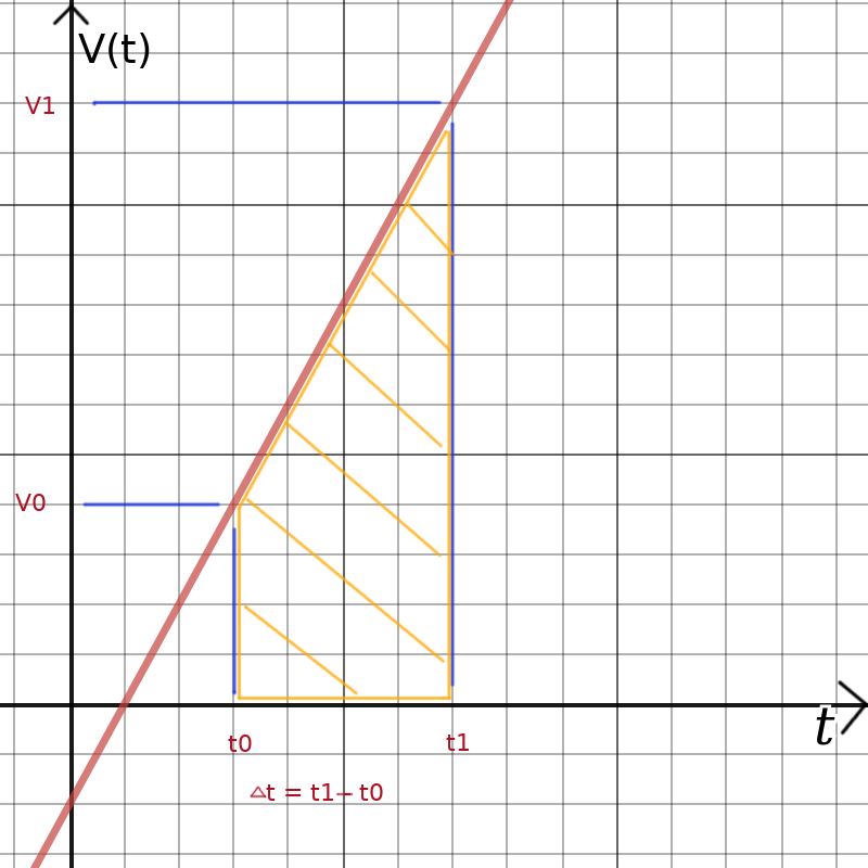
The term ∫v(t)∂t would be the area marked in orange. That area is:
v0 Δt + ½ (v1 - v0)Δt = ½ (v0 + v)Δt
Replacing ∫v(t)∂t with ½ (v0 + v)Δt results in the second high school equation.
It is also possible to do this purely mathematically and not graphically but that is a longer calculation which you can follow >here< if you want.
The second high school equation
Sorry, I am out of time. To be done later.
© 2004-2026 Guido Socher